Introduction

This article details the bottleneck of the Pandas rolling correlation function and presents our approach to solving it. Rolling correlation is a very powerful Pandas function that can be performed on a DataFrame or Series. However, we have found that the DataFrame.rolling().agg('corr') function is very slow when dealing with a large number of columns. Even when performing rolling operations on a DataFrame with empty rows but non-empty columns, it can still take a significant amount of time. More details is shown in Xorbits/issues.

We analyze the impact of different input shape on the performance of DataFrame.rolling(window=30).agg('corr') and use the py-spy package to visualize the time consumption of different functions through a flame graph.

Performance Testing

We use Huge Stock Market Dataset as test data, which records Historical daily prices and volumes of all U.S. stocks and ETFs. By selecting 1000 stocks’ returns to generate a csv file returns.csv.

            bac_i.us    glt.us    ...    atu.us    jhy.us    xco.us    mik.us    apf.us
2015-01-01       NaN       NaN    ...       NaN       NaN       NaN       NaN       NaN
2015-01-02       NaN       NaN    ...       NaN       NaN       NaN       NaN       NaN
2015-01-03  0.000000  0.000000    ...  0.000000       NaN  0.000000  0.000000  0.000000
2015-01-04  0.000000  0.000000    ...  0.000000       NaN  0.000000  0.000000  0.000000
2015-01-05 -0.003401 -0.034154    ... -0.032051       NaN -0.038278 -0.039271 -0.004082
...              ...       ...    ...       ...       ...       ...       ...       ...
2015-12-27  0.000000  0.000000    ...  0.000000  0.000000  0.000000  0.000000  0.000000
2015-12-28  0.005668 -0.023806    ... -0.016163  0.005981  0.035398  0.008692 -0.001392
2015-12-29  0.003322  0.024944    ...  0.017664 -0.007005  0.025641  0.006349 -0.001467
2015-12-30 -0.002976 -0.015136    ... -0.019380  0.001269 -0.100000 -0.004056 -0.004041
2015-12-31 -0.001493 -0.023771    ... -0.014771 -0.008246  0.148148  0.000452  0.009147

[365 rows x 1000 columns]

With dataset (365, 1000)

import pandas as pd
import time
return_matrix = pd.read_csv("/path/to/returns.csv", index_col=0, parse_dates=True)
roll = return_matrix.rolling(window=30).agg('corr')

Execution time: 105.7209062576294

With horizontal half (182, 1000)

import pandas as pd
import time
return_matrix = pd.read_csv("/path/to/returns.csv", index_col=0, parse_dates=True)
return_matrix = return_matrix.iloc[: len(return_matrix) // 2]
roll = return_matrix.rolling(window=30).agg('corr')

Execution time: 97.95154094696045

With vertical half (365, 500)

import pandas as pd
import time
return_matrix = pd.read_csv("/path/to/returns.csv", index_col=0, parse_dates=True)
return_matrix = return_matrix[return_matrix.columns[: 500]]
roll = return_matrix.rolling(window=30).agg('corr')

Execution time: 26.112659215927124

With empty dataset (0, 1000)

import pandas as pd
import time
return_matrix = pd.read_csv("/path/to/returns.csv", index_col=0, parse_dates=True)
return_matrix = return_matrix.drop(return_matrix.index)
roll = return_matrix.rolling(window=30).agg('corr')

Execution time: 89.09344792366028

The experiments above shows that the execution time of rolling correlation on dataframes is largely dependent on the number of columns, rather than the number of rows.

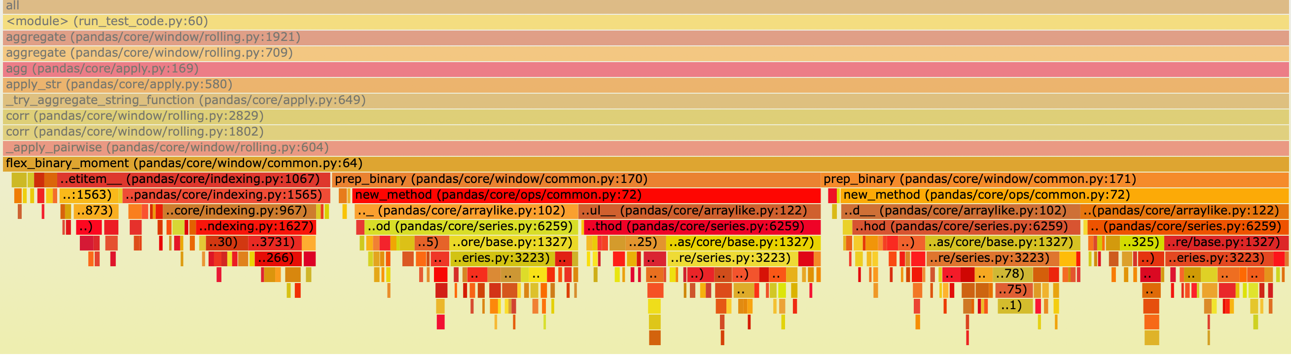
We use the py-spy package to visualize the time consumption of different modules as follows:

The main execution time is concentrated in the following function

def flex_binary_moment(arg1, arg2, f, pairwise=False):
    results = defaultdict(dict)
    for i in range(len(arg1.columns)):
        for j in range(len(arg2.columns)):
            if j < i and arg2 is arg1:
                # Symmetric case
                results[i][j] = results[j][i]
            else:
                results[i][j] = f(
                    *prep_binary(arg1.iloc[:, i], arg2.iloc[:, j])
                )

flex_binary_moment is used to calculate the rolling correlation between every two columns. results[i][j] represents the rolling correlation between the i-th and j-th columns. The two time-consuming parts of flex_binary_moment are f() (35.5%) and prep_binary(57.2%). f() calculates the rolling correlation, while prep_binary masks out rows with NaN values in the two columns.

Some people may wonder why the time taken to calculate the rolling correlation is shorter than that of prep_binary. Let’s take a look at the code for the two parts below.

prep_binary

def prep_binary(arg1, arg2):
    # mask out values, this also makes a common index...
    X = arg1 + 0 * arg2
    Y = arg2 + 0 * arg1

    return X, Y

Here’s the flame graph of prep_binary execution, which shows that a significant amount of time is spent on calculating X and Y.

rolling correlation

def corr_func(x, y):
    x_array = self._prep_values(x)
    y_array = self._prep_values(y)
    window_indexer = self._get_window_indexer()
    min_periods = (
        self.min_periods
        if self.min_periods is not None
        else window_indexer.window_size
    )
    start, end = window_indexer.get_window_bounds(
        num_values=len(x_array),
        min_periods=min_periods,
        center=self.center,
        closed=self.closed,
        step=self.step,
    )
    self._check_window_bounds(start, end, len(x_array))

    with np.errstate(all="ignore"):
        mean_x_y = window_aggregations.roll_mean(
            x_array * y_array, start, end, min_periods
        )
        mean_x = window_aggregations.roll_mean(x_array, start, end, min_periods)
        mean_y = window_aggregations.roll_mean(y_array, start, end, min_periods)
        count_x_y = window_aggregations.roll_sum(
            notna(x_array + y_array).astype(np.float64), start, end, 0
        )
        x_var = window_aggregations.roll_var(
            x_array, start, end, min_periods, ddof
        )
        y_var = window_aggregations.roll_var(
            y_array, start, end, min_periods, ddof
        )
        numerator = (mean_x_y - mean_x * mean_y) * (
            count_x_y / (count_x_y - ddof)
        )
        denominator = (x_var * y_var) ** 0.5
        result = numerator / denominator
    return Series(result, index=x.index, name=x.name)

The key here is that Pandas convert x_array and y_array to numpy arrays for Cython routines.

x_array = _prep_values(x)
y_array = _prep_values(y)

Solution

A simple optimization method from a parallel perspective is proposed, and as analyzed earlier, reducing the columns significantly helps to reduce the computation time. Assuming a DataFrame of shape (365, N) and a parallelism degree of m, m Sub-DataFrames can be generated with a shape of (365, N/m). The parallelism degree can be set to the number of cores of the processor. To simplify the process, communication time between different cores is ignored and the original DataFrame is broadcasted to each core before the calculation.

Without adding any parallel strategy, the computational complexity is:

C_1 = N^2

With any parallel strategy, since each core can operate simultaneously, the number of computations is:

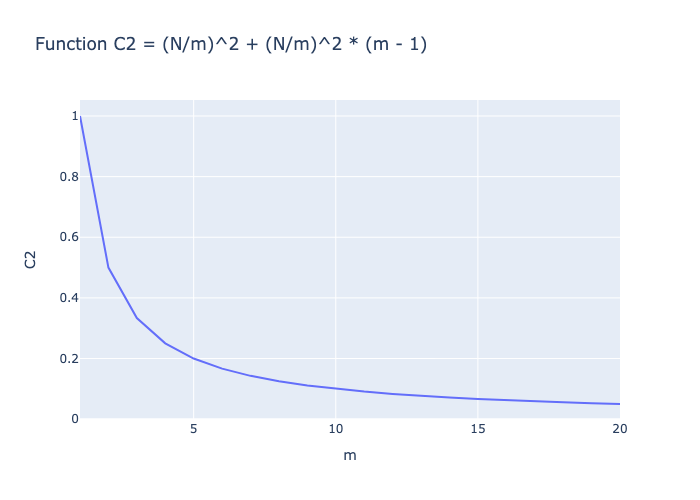
C_2 = (N/m)^2 + (N/m)^2 * (m - 1)

In C2, the first term is the required computation for the current Sub-DataFrame, and the second term is the required computation for the current Sub-DataFrame and other Sub-DataFrames. As can be seen, the computation is reduced after parallelization.

The following figure illustrates the change of computational complexity as the value of m increases.

Conclusion

This study identified a performance issue associated with DataFrame.rolling().agg('corr') and utilized the py-spy module to generate a flame graph that visualizes time consumption by various modules. Our analysis revealed that the root cause of the performance issue was the index alignment operation of two arrays in the prep_binary function. Additionally, a simple optimization method was proposed from a parallel perspective. We anticipate that this study will offer assistance to developers focused on optimizing large-scale data computations with Pandas.